DeepSeek-V3(一):稀疏注意力机制(DSA)

这是 GPT 生成的内容。超过现有数学基础,只能说大概看懂了,后面基础上来了再细节推导和检查正确性。

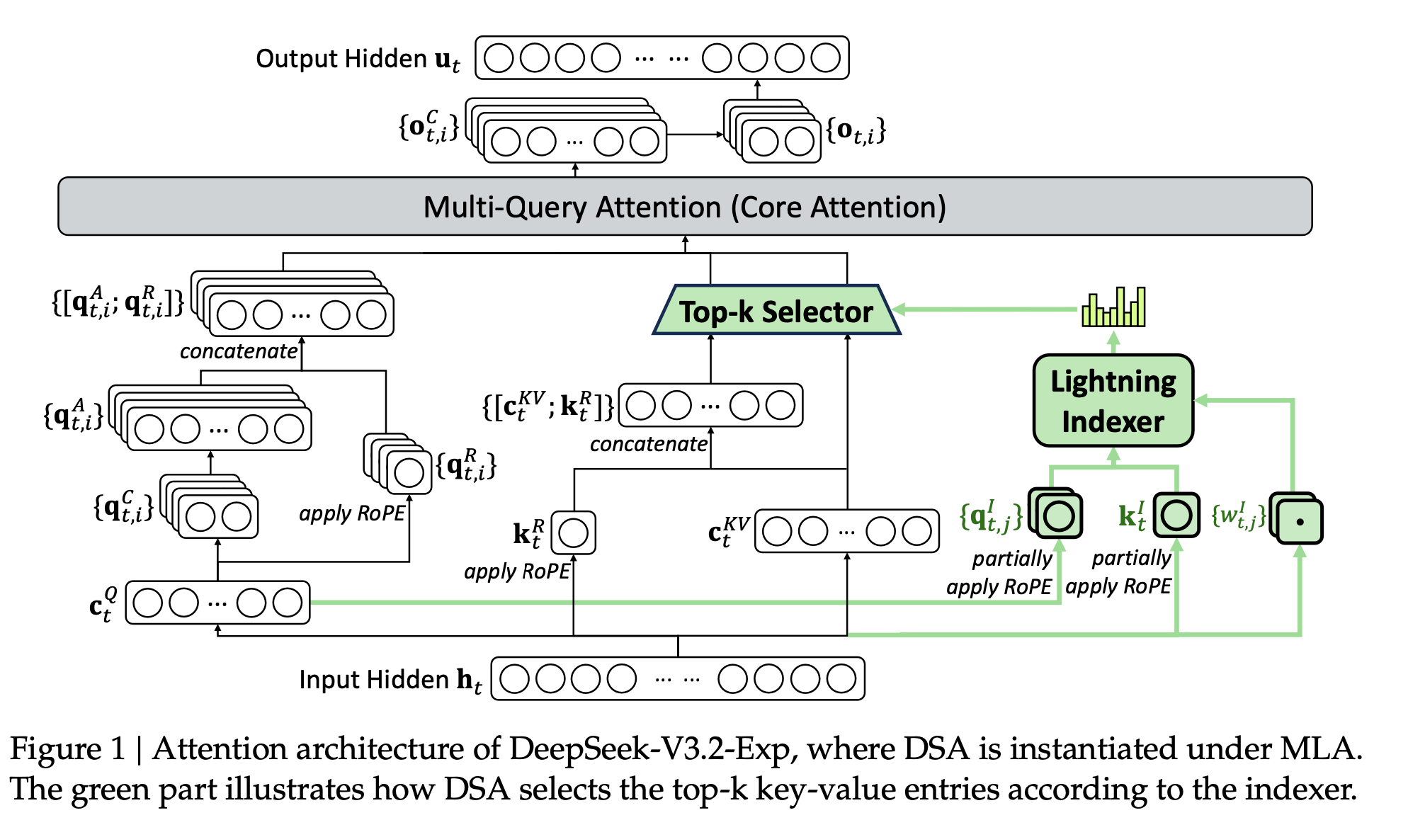
DeepSeek Sparse Attention, DSA 可以理解为一个两阶段稀疏注意力系统:

  1. 用一个很轻量的 Lightning Indexer 近似估计“哪些历史 token 对当前 query 重要”;
  2. 再用 Fine-grained Sparse Attention 只对被选中的少量 token 做真正的 softmax attention。

其目标是把标准注意力的复杂度从近似

$$ O(n^2 d) $$

降低到

$$ O(n k d) + O(\text{indexing cost}), $$

其中 $n$ 是序列长度,$d$ 是 hidden/head 维度,$k \ll n$ 是每个 query 选中的 key/value 数量。DeepSeek-V3.2 技术报告中将 DSA 作为长上下文效率机制引入,并包含 Lightning Indexer 与 fine-grained sparse attention 的训练/部署流程[1]。后续工作也指出,token-level sparse attention 中 indexer 本身会成为瓶颈,因此专门研究了更高效的层次化 indexer[2]


1. 标准 dense attention 回顾

设某一层、某一 attention head 中:

$$ Q = XW_Q \in \mathbb{R}^{n \times d}, \quad K = XW_K \in \mathbb{R}^{n \times d}, \quad V = XW_V \in \mathbb{R}^{n \times d}. $$

第 $i$ 个 query token 对所有历史 key 的注意力为:

$$ \alpha_{ij} = \frac{ \exp(q_i^\top k_j / \sqrt d) }{ \sum_{\ell \le i} \exp(q_i^\top k_\ell / \sqrt d) }, \quad j \le i. $$

输出为:

$$ o_i = \sum_{j \le i} \alpha_{ij} v_j. $$

问题是,对每个 $i$,都要计算 $q_i^\top k_j$,其中 $j = 1,\dots,i$。总复杂度为:

$$ \sum_{i=1}^{n} O(i d) = O(n^2 d). $$

长上下文下,例如 (n = 128K),dense attention 的代价非常高。


2. DSA 的核心思想

DSA 的核心是:不要对所有 key 做精确 attention,而是先用便宜的 indexer 找候选 key。

也就是说,对于每个 query $q_i$,我们不再使用所有历史 token 集合:

$$ \mathcal{P}_i = \{1,2,\dots,i\}, $$

而是选择一个稀疏子集:

$$ \mathcal{S}_i \subset \mathcal{P}_i, \quad |\mathcal{S}_i| = k, \quad k \ll i. $$

然后只在 $\mathcal{S}_i$ 上做 softmax:

$$ \alpha_{ij}^{\text{sparse}} = \frac{ \exp(q_i^\top k_j / \sqrt d) }{ \sum_{\ell \in \mathcal{S}_i} \exp(q_i^\top k_\ell / \sqrt d) }, \quad j \in \mathcal{S}_i. $$

输出:

$$ o_i^{\text{sparse}} = \sum_{j \in \mathcal{S}_i} \alpha_{ij}^{\text{sparse}} v_j. $$

所以 DSA 的关键数学问题变成:

$$ \mathcal{S}_i = \operatorname{TopK}_{j \le i} \bigl( \text{score}_{ij} \bigr), $$

其中 $\text{score}_{ij}$ 要尽可能接近真实 attention logit:

$$ q_i^\top k_j, $$

但计算成本必须远低于 $O(nd)$。


3. Lightning Indexer:用低成本分数近似真实 attention 重要性

3.1 标准 attention score

真实 attention 的未归一化分数是:

$$ s_{ij} = \frac{q_i^\top k_j}{\sqrt d}. $$

如果直接对所有 $j$ 计算 $s_{ij}$,那又回到了 dense attention。

因此 Lightning Indexer 引入一个轻量级映射:

$$ \phi_Q(q_i) \in \mathbb{R}^{r}, \quad \phi_K(k_j) \in \mathbb{R}^{r}, $$

其中

$$ r \ll d. $$

然后用低维内积估计重要性:

$$ \hat{s}_{ij} = \phi_Q(q_i)^\top \phi_K(k_j). $$

如果 $\hat{s_{ij}}$ 与 $s_{ij}$ 排序一致性较强,那么我们可以用:

$$ \mathcal{S}_i = \operatorname{TopK}_{j \le i} \hat{s}_{ij} $$

代替

$$ \operatorname{TopK}_{j \le i} s_{ij}. $$

这就是 Lightning Indexer 的数学本质:
用便宜的近似打分函数预测真实 attention 的 Top-K 支持集。


3.2 低秩近似视角

假设真实 attention score 矩阵为:

$$ S = QK^\top \in \mathbb{R}^{n \times n}. $$

Lightning Indexer 试图构造一个低成本矩阵:

$$ \hat{S} = \tilde{Q}\tilde{K}^\top, $$

其中:

$$ \tilde{Q} = Q A \in \mathbb{R}^{n \times r}, \quad \tilde{K} = K B \in \mathbb{R}^{n \times r}, $$

并且 $r \ll d$。

于是:

$$ \hat{S}_{ij} = (QA)_i^\top (KB)_j. $$

如果 $A,B$ 是可学习参数,则 indexer 可以通过训练学习如何预测 dense attention 的重要 token。

理想目标可以写成:

$$ \operatorname{TopK}(S_i) \approx \operatorname{TopK}(\hat{S}_i). $$

这里 $S_i$ 表示第 $i$ 行,也就是第 $i$ 个 query 对所有 key 的真实 attention logits。


4. Lightning Indexer 的训练目标

为了让 indexer 选出的 token 接近 dense attention,可以设计若干训练目标。DeepSeek-V3.2 报告中提到会先进行 indexer warm-up,然后再引入 fine-grained sparse attention[1:1]。从数学上,可以理解为先让 indexer 学会模仿 dense attention 的选择分布。

4.1 以 dense attention 为 teacher

设 dense attention 分布为:

$$ p_{ij} = \frac{\exp(s_{ij})}{\sum_{\ell \le i}\exp(s_{i\ell})}. $$

Indexer 产生的近似分布为:

$$ \hat{p}_{ij} = \frac{\exp(\hat{s}_{ij})}{\sum_{\ell \le i}\exp(\hat{s}_{i\ell})}. $$

一个自然的训练目标是 KL 散度:

$$ \mathcal{L}_{\text{index}} = \sum_i \operatorname{KL} \left( p_i \;||\; \hat{p}_i \right). $$

展开为:

$$ \mathcal{L}_{\text{index}} = \sum_i \sum_{j \le i} p_{ij} \log \frac{p_{ij}}{\hat{p}_{ij}}. $$

这个目标鼓励 indexer 的排序和 dense attention 接近。


4.2 Top-K 集合匹配目标

因为 sparse attention 最终关心的是 Top-K 选择,而不是完整分布,所以也可以用集合匹配的思想。

设 dense attention 的真实 Top-K 集合为:

$$ \mathcal{T}_i = \operatorname{TopK}_{j \le i}(s_{ij}). $$

Indexer 选出的集合为:

$$ \mathcal{S}_i = \operatorname{TopK}_{j \le i}(\hat{s}_{ij}). $$

希望最大化 recall:

$$ \operatorname{Recall}_i = \frac{ |\mathcal{S}_i \cap \mathcal{T}_i| }{ |\mathcal{T}_i| }. $$

对应的目标是:

$$ \max \sum_i \frac{ |\mathcal{S}_i \cap \mathcal{T}_i| }{ k }. $$

实际训练中,Top-K 操作不可微,所以通常会用 soft surrogate,例如 pairwise ranking loss:

$$ \mathcal{L}_{\text{rank}} = \sum_i \sum_{j \in \mathcal{T}_i} \sum_{m \notin \mathcal{T}_i} \max \left( 0, \gamma - \hat{s}_{ij} + \hat{s}_{im} \right), $$

其中 $\gamma > 0$ 是 margin。
这个损失要求真正重要的 token $j$ 的 indexer score 高于不重要 token $m$。


5. Fine-grained Sparse Attention

Lightning Indexer 只负责“找候选”。真正输出仍然由标准 attention 公式计算,只不过注意力范围缩小到 $\mathcal{S}_i$。

即:

$$ \mathcal{S}_i = \operatorname{TopK}_{j \le i} \hat{s}_{ij}. $$

然后在这个集合上计算真实 logit:

$$ s_{ij} = \frac{q_i^\top k_j}{\sqrt d}, \quad j \in \mathcal{S}_i. $$

再做局部 softmax:

$$ \alpha_{ij}^{\text{DSA}} = \frac{ \exp(s_{ij}) }{ \sum_{\ell \in \mathcal{S}_i} \exp(s_{i\ell}) }, \quad j \in \mathcal{S}_i. $$

输出:

$$ o_i^{\text{DSA}} = \sum_{j \in \mathcal{S}_i} \alpha_{ij}^{\text{DSA}} v_j. $$

注意这里有一个重要区别:

  • Indexer score $\hat{s}_{ij}$:只用于选择 token;
  • 真实 attention score $s_{ij}$:用于最终 softmax 和加权求和。

所以 DSA 不是简单地用近似 attention 替代原 attention,而是:

$$ \text{cheap indexer for retrieval} + \text{exact attention over retrieved tokens}. $$

这也是它比纯近似 attention 更稳的原因。


6. 为什么叫 Fine-grained?

很多 sparse attention 方法是 block-level 的,比如把上下文分成 block:

$$ B_1, B_2, \dots, B_m. $$

然后选择若干 block:

$$ \mathcal{B}_i = \operatorname{TopKBlock}(q_i). $$

这种方法粒度较粗。如果 block 大小为 $b$,选中一个 block 就必须计算其中所有 $b$ 个 token,即使其中大多数并不重要。

Fine-grained sparse attention 则直接在 token 级别选:

$$ \mathcal{S}_i = \{j_1, j_2, \dots, j_k\}. $$

这比 block-level 更精细:

$$ \text{block-level: select blocks} $$
$$ \text{fine-grained: select individual tokens}. $$

好处是:

$$ k_{\text{token}} \ll k_{\text{block}} \cdot b $$

时,计算更省。

但坏处是 indexer 压力更大:
因为每个 query 都要在大量历史 token 中找 Top-K。后续 HISA 等工作正是指出 fine-grained token-level sparse attention 中 indexer 会成为新的瓶颈,并提出层次化索引来缓解[2:1]


7. DSA 的整体计算流程

对于当前 query token $i$:

Step 1:计算 query/key/value

$$ q_i = x_i W_Q, \quad k_j = x_j W_K, \quad v_j = x_j W_V. $$

Step 2:Lightning Indexer 生成低维表示

$$ \tilde{q}_i = \phi_Q(q_i), \quad \tilde{k}_j = \phi_K(k_j). $$

其中:

$$ \tilde{q}_i,\tilde{k}_j \in \mathbb{R}^{r}, \quad r \ll d. $$

Step 3:计算 indexer score

$$ \hat{s}_{ij} = \tilde{q}_i^\top \tilde{k}_j. $$

Step 4:选出 Top-K token

$$ \mathcal{S}_i = \operatorname{TopK}_{j \le i} \hat{s}_{ij}. $$

Step 5:对选中 token 做真实 attention

$$ s_{ij} = \frac{q_i^\top k_j}{\sqrt d}, \quad j \in \mathcal{S}_i. $$
$$ \alpha_{ij} = \frac{ \exp(s_{ij}) }{ \sum_{\ell \in \mathcal{S}_i} \exp(s_{i\ell}) }. $$

Step 6:聚合 value

$$ o_i = \sum_{j \in \mathcal{S}_i} \alpha_{ij} v_j. $$

8. 复杂度推导

8.1 Dense attention

每个 query 对 $i$ 个 key 计算内积,每个内积维度为 $d$:

$$ C_{\text{dense}} = \sum_{i=1}^{n} i d = \frac{n(n+1)}{2}d = O(n^2 d). $$

8.2 DSA attention 主体复杂度

如果每个 query 只选 $k$ 个 key:

$$ C_{\text{attn}} = \sum_{i=1}^{n} k d = O(n k d). $$

其中 $k \ll n$。


8.3 Indexer 复杂度

若 Lightning Indexer 使用低维维度 $r$,粗略计算所有 query-key index score 的成本为:

$$ C_{\text{index}} = O(n^2 r). $$

因为 $r \ll d$,它比 dense attention 便宜。

但如果真的计算全量 $n^2$ 个 index score,在极长上下文下仍然很贵。因此实际系统通常还需要结合:

  • 分块;
  • 层次化索引;
  • 缓存;
  • 近似 Top-K;
  • 局部窗口加全局检索;
  • query 分组;
  • hardware-aware kernel。

后续研究如 HISA 就指出 DSA 这类 token-level sparse attention 的 indexer 会成为新瓶颈,因此提出 hierarchical indexing 来进一步降低 indexer 代价[2:2]


9. 误差分析:DSA 近似 dense attention 的条件

Dense attention 输出为:

$$ o_i = \sum_{j \le i} p_{ij} v_j. $$

DSA 输出为:

$$ \hat{o}_i = \sum_{j \in \mathcal{S}_i} \hat{p}_{ij} v_j, $$

其中:

$$ \hat{p}_{ij} = \frac{ \exp(s_{ij}) }{ \sum_{\ell \in \mathcal{S}_i} \exp(s_{i\ell}) }. $$

设未被选中的集合为:

$$ \mathcal{R}_i = \mathcal{P}_i \setminus \mathcal{S}_i. $$

dense attention 在被丢弃 token 上的总概率质量为:

$$ \epsilon_i = \sum_{j \in \mathcal{R}_i} p_{ij}. $$

如果 $\epsilon_i$ 很小,则 sparse attention 近似 dense attention 较好。

换句话说,DSA 成功的关键是:

$$ \sum_{j \notin \mathcal{S}_i} p_{ij} \approx 0. $$

也就是 indexer 选中的 token 覆盖了 dense attention 的大部分概率质量。

可以给出一个直觉误差界。假设:

$$ \|v_j\| \le M. $$

那么丢弃部分导致的误差大致受控于:

$$ \left\| \sum_{j \in \mathcal{R}_i} p_{ij} v_j \right\| \le \sum_{j \in \mathcal{R}_i} p_{ij} \|v_j\| \le M \epsilon_i. $$

因此,如果 indexer 能让 $\epsilon_i$ 很小,DSA 输出就接近 dense attention。


10. 为什么需要 warm-up?

如果一开始就让模型使用 sparse attention,indexer 还没学会选 token,可能会漏掉重要上下文,训练不稳定。

所以可以先进行 indexer warm-up:

  1. 主模型仍然使用 dense attention;
  2. 同时训练 Lightning Indexer 去预测 dense attention 的重要 token;
  3. 当 indexer 的 Top-K recall 足够高后,再切换到 fine-grained sparse attention。

数学上就是先优化:

$$ \mathcal{L}_{\text{index}} $$

让:

$$ \operatorname{TopK}(\hat{s}_{ij}) \approx \operatorname{TopK}(s_{ij}), $$

再优化完整语言模型损失:

$$ \mathcal{L}_{\text{LM}} = -\sum_t \log p(x_t | x_{<t}). $$

最终训练目标可以看成:

$$ \mathcal{L} = \mathcal{L}_{\text{LM}} + \lambda \mathcal{L}_{\text{index}}, $$

其中 $\lambda$ 控制 indexer 监督强度。


11. 一个简化伪代码

# Q, K, V: [n, d]
# Wq_idx, Wk_idx: indexer projection, d -> r
# k_select: number of selected tokens

Q_idx = Q @ Wq_idx      # [n, r]
K_idx = K @ Wk_idx      # [n, r]

outputs = []

for i in range(n):
    # causal keys: 0 ... i
    idx_scores = Q_idx[i] @ K_idx[:i+1].T      # [i+1]

    # select fine-grained token indices
    S_i = topk(idx_scores, k=k_select)

    # exact attention over selected tokens
    logits = Q[i] @ K[S_i].T / sqrt(d)         # [k]
    attn = softmax(logits)

    out = attn @ V[S_i]                       # [d]
    outputs.append(out)

这个伪代码对应数学公式:

$$ \mathcal{S}_i = \operatorname{TopK} \left( \tilde{q}_i^\top \tilde{k}_j \right), $$
$$ o_i = \sum_{j \in \mathcal{S}_i} \operatorname{softmax} \left( \frac{q_i^\top k_j}{\sqrt d} \right) v_j. $$

12. 总结

DeepSeek Sparse Attention = 学习型 token 级检索器 + 精确子集注意力。

更形式化地说:

$$ \boxed{ \mathcal{S}_i = \operatorname{TopK}_{j \le i} \left( \phi_Q(q_i)^\top \phi_K(k_j) \right) } $$
$$ \boxed{ o_i = \sum_{j \in \mathcal{S}_i} \frac{ \exp(q_i^\top k_j / \sqrt d) }{ \sum_{\ell \in \mathcal{S}_i} \exp(q_i^\top k_\ell / \sqrt d) } v_j } $$

Lightning Indexer 负责便宜地找 $\mathcal{S}_i$,Fine-grained Sparse Attention 负责在 $\mathcal{S}_i$ 上做真实 attention。只要 indexer 能保证被丢弃 token 的 attention mass 很小:

$$ \epsilon_i = \sum_{j \notin \mathcal{S}_i} p_{ij} \ll 1, $$

则 DSA 可以在保持效果的同时把主要 attention 计算从:

$$ O(n^2 d) $$

降到:

$$ O(n k d) + O(\text{indexer}). $$

评论